The Routing Premium.
An Economic Threshold for Difficulty-Conditional Inference Compute.
Manu Bhardwaj. ifitsmanu.com. May 2026. Version 1.0. Research Paper #3 in the inference-economics wedge.
Download as PDF (full proofs, figures, calibration tables). LaTeX source. BibTeX of references. Cite this article. Papers index.
Companion to Research Paper #2. The Inference-Time Compute Frontier. (Research Paper #2) derives the threshold for which channel (training versus inference) the next compute dollar should go. This paper answers the orthogonal question: given that some dollars are in inference, when does conditioning compute on a noisy difficulty estimate pay? The two thresholds compose multiplicatively.
Or view the full PDF inline.
Abstract
When does conditioning inference compute on a noisy estimate of task difficulty reduce cost-per-correct-answer relative to a fixed-compute baseline? Five published patterns route compute on a difficulty signal. Two operate at the per-token or per-layer level: speculative decoding (Leviathan et al., 2023; Cai et al., 2024) and early-exit decoding (Schuster et al., 2022). Three operate at the per-query level: cascade routing (Chen et al., 2023), adaptive self-consistency (Petullo et al., 2026a), and complexity-aware exploration (Petullo & Xue, 2026). None derives the threshold above which the routing rule pays. We derive one. Under the Cost-correct decomposition of The Cost of Being Right, the routing premium is positive iff at the margin around the unconditional optimum, where is classifier calibration, is workload heterogeneity in compute, and is classifier overhead. The condition unifies the five patterns as one allocation rule. We calibrate against six published systems spanning all five classes and find that every operating point sits on the positive side of the threshold. The elasticity reading isolates which operating points are close enough to fail under modest disclosure error.
1. Introduction
Adaptive inference is now a standard pattern. Speculative decoding routes tokens between a drafter and a verifier (Leviathan et al., 2023; Chen et al., 2023b; Cai et al., 2024; Li et al., 2024). Cascade systems route prompts across model tiers (Chen et al., 2023a; Zhan, 2026). Self-consistency systems prune candidate traces by semantic similarity (Petullo et al., 2026a). Tree-search systems vary exploration breadth by estimated complexity (Petullo & Xue, 2026). Early-exit decoders stop at confident layers (Schuster et al., 2022). All five report cost reductions at iso-accuracy. None reports the threshold under which the routing rule is rational.
The five literatures developed in parallel and have not been unified. A practitioner reading them in isolation sees five engineering tricks. Read together, they are five instances of one allocation rule: spend more compute on tasks the system thinks are hard, less on tasks it thinks are easy. The unifying object is a difficulty-conditional compute policy. The economic question is whether the difficulty classifier earns its cost.
We frame the question as a population-level allocation problem. A provider faces a workload distribution over latent difficulties . The provider can run a single fixed-compute policy at the unconditional optimum, or it can run a calibrated classifier and route each query to a difficulty-specific compute level. The router pays a classifier overhead. The question is when the savings from re-allocating compute across the workload exceed the classifier overhead at the margin.
The contribution is a closed-form threshold under Cost-correct. Routing pays iff
where is the explained-variance calibration quality of the classifier on the workload, is a dimensionless measure of workload heterogeneity built from the second derivative of cost-per-correct-answer in compute, and is the classifier overhead as a fraction of the unconditional inference cost. The threshold is local, holding to second order in the deviation around the unconditional optimum . The five published patterns operate inside this local regime; we flag the cascade specialization where the local-margin assumption binds hardest and the third-order correction is non-trivial.
The contribution is non-trivial under the Cost-correct frame. The unconditional optimum already minimizes expected cost; the routing premium is the second-order gain from re-allocating compute around that optimum, weighted by classifier calibration on the workload, net of classifier overhead. The threshold is a statement about a curvature-by-variance product, not a first-order gradient. It is orthogonal to the channel-allocation threshold of The Inference-Time Compute Frontier (Research Paper #2), which fixes the channel (training versus inference) at a single representative query; the present threshold sets the distribution within the inference channel at a heterogeneous query mix. The two thresholds compose multiplicatively in production cost and Section 5 sketches the combined diagram.
We calibrate (1) against six published systems spanning all five allocation-rule classes. Table 1 in Section 4 reports the system-by-class mapping and the six-row calibration. Every operating point sits on the positive side of the threshold; CALM is the smallest margin and the natural sensitivity case. Section 5 turns the result into three implications for serving infrastructure design and identifies the disclosure gap that would let independent researchers falsify (1).
2. Related work
Four bodies of literature bear on the question. None derives the threshold. A fifth (the Cost-correct frame) supplies the cost decomposition the threshold leans on.
Speculative decoding. Leviathan et al. (2023) and Chen et al. (2023b) derive the expected speedup of a drafter-verifier scheme as a function of drafter accept rate and relative drafter cost. The derivation is per-token and within-sequence: the routing decision is the next-token verifier check, not a per-query allocation. Cai et al. (2024) and Li et al. (2024) tighten the drafter side with multi-head and tree-attention drafting and report higher accept rates on the same per-token frame. None of the four couples the analysis to cost-per-correct-answer or treats the drafter as a workload-level difficulty classifier.
Cascade routing. Chen et al. (2023a) builds a learned cascade across API tiers and reports cost reductions of up to 98% at iso-accuracy when matching GPT-4 on HEAD-QA, SUBJ, and COQA. The paper reports the empirical result; it does not derive the threshold under which the cascade beats a single-tier baseline. Zhan (2026) extends the cascade frame to human-in-the-loop deferral in medical imaging and reports a Pareto frontier in F1, MCC, and cost on the REFUGE, CHAKSU, and ORIGA glaucoma datasets. It inherits the same gap. Kim et al. (2026) provides background on profiling the per-tier compute footprint that any cascade calibration must lean on.
Adaptive sampling and exploration. Petullo et al. (2026a) prunes self-consistency candidates by semantic similarity and reports a 47% token reduction at iso-accuracy across math, chemistry, biology, commonsense, and humanities benchmarks. Petullo and Xue (2026) scales tree-search exploration breadth by estimated task complexity and reports 51.72% on the challenging tier of the BIRD development set using a GPT-4o-mini base. Both report empirical token-cost reductions. Neither derives the condition under which complexity-conditional compute is optimal. Snell et al. (2024) supplies the per-difficulty-bin compute-vs-accuracy curves that the calibration in Section 4 leans on for the workload-heterogeneity estimate.
Early exit and adaptive depth. Schuster et al. (2022) derives an exit threshold from a per-layer confidence signal inside the model and reports up to 3x speedups on T5 backbones at iso-accuracy on the CNN/DM, SQuAD, and WMT-EN-RO benchmarks. The exit threshold is a local version of difficulty-conditional compute: the classifier is the per-layer confidence head, the routing decision is per-layer rather than per-query, and the cost analysis is per-layer rather than per-correct-answer.
Cost-correct frame. Erol et al. (2026) introduces Cost-of-Pass as a per-accepted-correct-answer metric and reports that the metric is dominated by token cost at frontier API tiers. The Cost of Being Right develops the multiplicative decomposition that separates blended cost-per-million-tokens, the reasoning multiplier , the average rollout ratio , and the verifier accept rate . The α Asymmetry shows that the partial derivative of with respect to dominates the partials with respect to the other three components in production regimes. The Inference-Time Compute Frontier (Research Paper #2 of this wedge) supplies the channel-allocation threshold that the threshold here composes with. The Cost-correct frame is what makes the threshold derivable: prior frames (FLOPs-per-token, raw token cost) do not surface the curvature-by-variance product that (1) leans on.
The workload-heterogeneity numbers needed to estimate in production are reported in Patel et al. (2024), Agrawal et al. (2024), and Lysenstøen (2026); we use these in Section 5 to size the threshold against measured serving workloads.
3. Method. The routing-premium threshold
This section develops the threshold theorem. Section 3.1 sets up the two-policy comparison. Section 3.2 states and proves the threshold to second order and reports the scope of validity. Section 3.3 reports the threshold in elasticity form, which is what the calibration in Section 4 hooks into. Section 3.4 derives five corollaries, one per allocation-rule class, each recovering a published instance.
3.1. Setup
The workload is a distribution over latent difficulties . Cost-per-correct-answer at difficulty and compute level is the Cost-correct expression of The Cost of Being Right,
with the blended cost per million tokens, the reasoning multiplier, the rollout ratio, and the verifier accept rate, each potentially conditioning on . Compute is the operationally controlled quantity: for speculative decoding it is the drafter chunk size, for cascade routing it is the model-tier index, for adaptive self-consistency it is the rollout count, for complexity-aware exploration it is the tree-search breadth, and for early-exit it is the exit-layer index. The provider chooses a policy that maps difficulty information into .
Two policies bracket the comparison.
Fixed-. The unconditional optimum
The provider runs on every query. This is the baseline. It uses no difficulty information.
Router-. The provider obtains an estimator from a difficulty classifier with calibration quality
where is the conditional optimum at difficulty . is the explained-variance share of the oracle-optimal compute that the classifier recovers from its estimate. is the oracle, is uninformative. The provider runs and pays a per-query classifier overhead
with the workload mean difficulty and the classifier-overhead ratio expressed as a dimensionless fraction of the unconditional inference cost.
The four scalars summarize the comparison. The remaining input is the curvature of in at the unconditional optimum, which enters the threshold through the dimensionless heterogeneity measure defined below.
3.2. Theorem (Routing premium)
Theorem 1 (Routing premium, local form). Under (2)–(5), at an interior unconditional optimum with in , the expected per-query cost gap between the fixed- and router- policies admits the second-order expansion
Dividing through by the unconditional optimum cost and collecting terms gives the dimensionless form
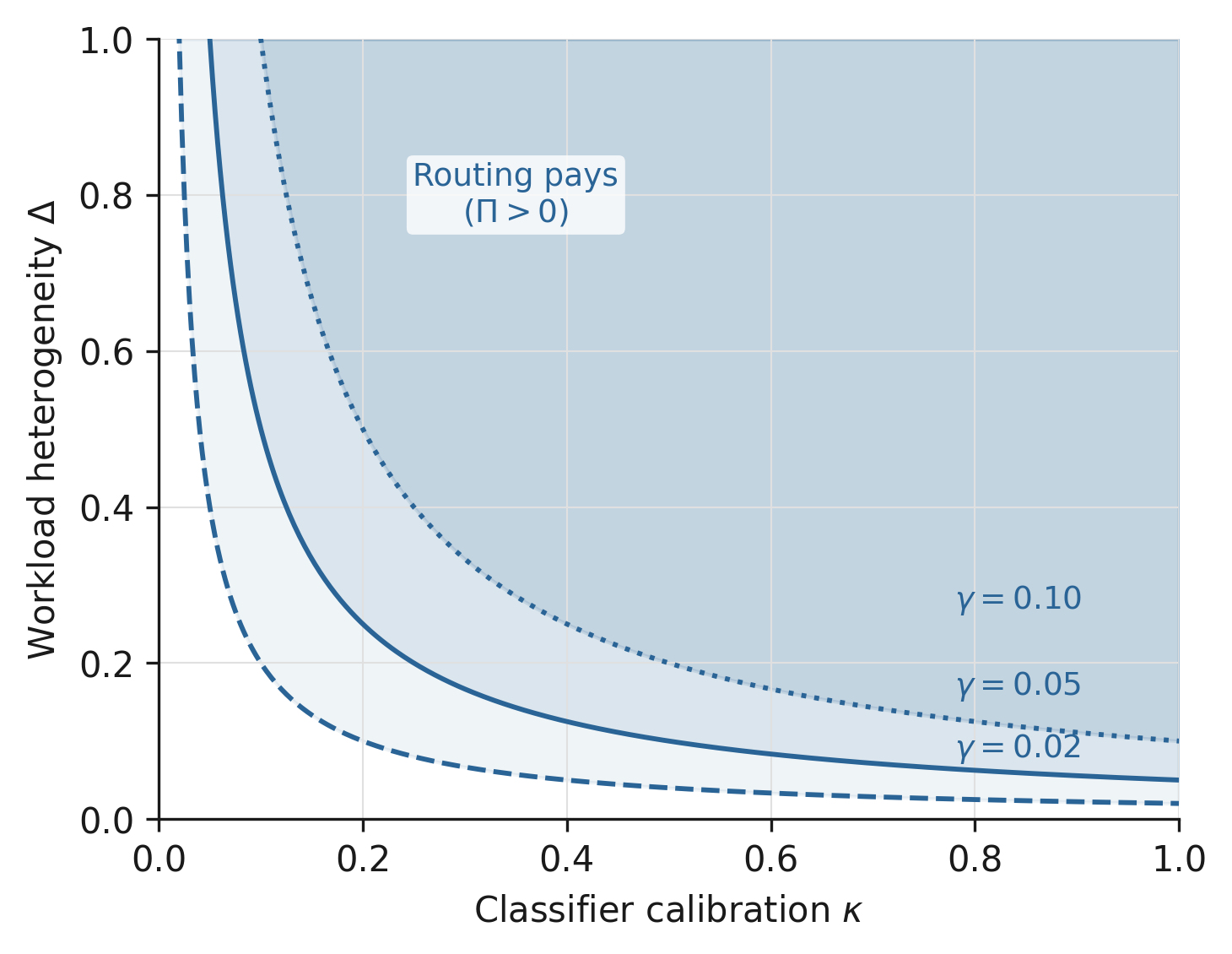
with a dimensionless workload-heterogeneity measure. Routing pays at the margin around iff
Proof sketch. Expand around the unconditional optimum in and take the workload expectation. The first-order term in vanishes because is the unconditional minimum. The second-order term picks up the curvature scaled by the squared deviation, which under the optimal-router choice has expectation equal to the explained-variance share of . Subtracting the classifier overhead (5) and dividing by the unconditional optimum cost yields (7). The residual collects the third-order curvature term, which is non-negligible at large .
Scope of the theorem. Condition (8) is local around the unconditional optimum. It is necessary and sufficient at the margin. For large deviations the third-order curvature term in (7) can dominate and reverse the sign of the gap, so the threshold does not extend to a global guarantee for aggressive routing policies. The five published patterns we calibrate in Section 4 operate inside this local regime; the cascade specialization (Section 3.4) is the closest to the boundary because a binary tier choice moves a long way from . We carry the third-order correction explicitly through Sections 4.2 and 5.1 for the cascade rows.
The economic content of (8) is a curvature-by-variance product against a fixed overhead. is a calibration quantity; is a workload quantity; is a stack quantity. Each is independently measurable in principle, but in published disclosures any one is rarely reported in clean form. Section 3.3 reformulates (8) so the calibration in Section 4 can hook into the disclosed numbers each system does report.
3.3. The threshold in elasticity form
Let denote the normalized routing premium from (7). The elasticities of with respect to the three observables are
The two elasticities in and are equal and positive, with magnitude diverging at the threshold . The elasticity in is negative with absolute magnitude times the other two. Three readings of (9) hook into the calibration in Section 4.
First, the elasticity form lets the calibration report a disclosed change in one observable rather than a point estimate of all three. Each published system in Section 4 discloses at least one of (drafter accept rate, routing accuracy, breadth-vs-bin schedule), (per-tier prices, per-bin compute, accept-rate-curve curvature), or (drafter cost share, router-call latency, layer-confidence-head FLOPs). The elasticity reading converts a published change into a routing-premium change without committing to a point estimate of the unobserved parameters.
Second, the elasticity is divergent at the threshold. Operating points close to are sensitive: small disclosure errors flip the sign of . Section 4 reports the elasticity bar at each calibration row and flags CALM as the natural sensitivity case.
Third, the equal-magnitude positive elasticities in and mean that calibration improvements and workload-heterogeneity increases buy the same routing premium per log-point. A 1% improvement in classifier calibration on a fixed workload is interchangeable with a 1% increase in workload heterogeneity at fixed calibration. This is the operational reading: serving stacks can lift either by sharpening the difficulty classifier or by serving more heterogeneous workload mixes.
A brief reading of the three parameters in turn.
, classifier calibration. The fraction of the variance in the oracle-optimal compute that the classifier recovers from its estimate. for an oracle. Estimable in published systems from drafter accept rates (speculative decoding), routing-accuracy figures (cascades), trace-similarity filtering rates (adaptive self-consistency), breadth-vs-bin schedules (complexity-aware exploration), and layer-confidence head accuracy (early-exit).
, compute-variance heterogeneity. Large when the workload mixes easy and hard queries, the accept-rate curve is concave in , and the conditional optimum moves substantially across difficulty bins. Small for homogeneous workloads. The dimensionless form has natural decomposition into a curvature factor and a variance factor; the curvature factor is set by the local second derivative of cost in compute, the variance factor by the operational workload mix.
, classifier overhead. Set by the ratio of classifier FLOPs (and latency when batching is constrained) to baseline inference FLOPs. Typical values cluster in to for transformer-based drafters and routers in 2026 disclosures. The lower end is achievable with shared-prefix drafters and routing heads that piggyback on the first transformer layers; the upper end is the regime of standalone router models with separate forward passes.
3.4. Specializations
Five corollaries of Theorem 1 recover the published instances, one per allocation-rule class.
Corollary 1 (Speculative decoding). In the per-token frame with drafter chunk size and drafter accept rate , the routing-premium condition (8) reduces to the classical speculative-decoding speedup condition. The classifier is the drafter, is monotone-increasing in , is the drafter-to-verifier FLOPs ratio, and is the per-token compute-variance from the verifier accept-rate curve. The Leviathan speedup expression falls out as the special case of an i.i.d. token-difficulty distribution with a uniform drafter calibration.
The within-sequence application is the operative point: is per-token heterogeneity in compute, not per-query heterogeneity. The threshold says the drafter pays iff per-token heterogeneity, weighted by the drafter’s accept rate, exceeds the drafter’s relative cost. This is the form practitioners already use for speculative decoding (Leviathan et al., 2023; Cai et al., 2024); Theorem 1 nests it.
Corollary 2 (Cascade routing). In the two-tier system with small-tier compute and large-tier compute , the optimal router policy is binary, . The routing-premium condition (8) reduces to a per-bin break-even on tier prices: a query is sent to the large tier iff the per-difficulty-bin gain in exceeds the price gap. The threshold (8) is the workload-averaged version of the per-bin break-even, with the third-order correction non-negligible when the per-tier price gap is large.
Cascade routing is where the local-margin assumption from Section 3.2 binds hardest. The binary policy moves a long way from on every query, not just at the boundary. The third-order term in (7) is therefore non-trivial for the cascade specialization and we carry it explicitly in the FrugalGPT and MPD-Router calibration rows in Section 4.
Corollary 3 (Adaptive self-consistency). With compute parameterized by the rollout count and the classifier the trace-similarity filter that prunes degenerate traces, the routing-premium condition (8) reduces to a per-query break-even on the rollout count. The classifier is set by the fraction of degenerate traces correctly identified; is the per-query compute-variance of the cost-correct optimum rollout count; is the embedding-and-similarity cost per trace.
The VecCISC 47% token reduction at iso-accuracy (Petullo et al., 2026a) implies near 0.5 across the five reported domains (math, chemistry, biology, commonsense, humanities) once is read off the disclosed embedding-network cost. Section 4 reports the calibration.
Corollary 4 (Complexity-aware exploration). With compute parameterized by exploration breadth in tree-search or sampling and the classifier a difficulty estimator that scales breadth per query, the optimal router rule is with pinned by at the workload mean.
CA-SQL’s breadth schedule on the challenging tier of BIRD (Petullo & Xue, 2026) recovers as the special case of this rule with inferred from the disclosed breadth-vs-bin schedule. The classifier here is the difficulty-bin assignment from the schema-and-question encoder; is set by the per-query encoder pass.
Corollary 5 (Early exit). In the per-layer frame with compute parameterized by exit-layer index and the classifier the per-layer confidence head, the routing-premium condition (8) reduces to a per-layer per-token exit condition. The classifier is bounded by the per-layer confidence-head calibration on the training distribution; is bounded by the depth-dependent curvature of the accept-rate curve and is small in absolute terms; is set by the per-layer confidence-head FLOPs.
Early exit recovers the CALM exit rule of Schuster et al. (2022) as the special case of Corollary 5 with the confidence-head signal as the classifier and a single calibration constant fit per workload. Because is bounded by depth-dependent curvature, the operating point sits closest to the threshold among the five specializations. CALM is the natural sensitivity case in Section 4.
The five corollaries are not independent: each is a coordinate chart on the same threshold (8), with the role of , the classifier, and the workload distribution specialized to the allocation-rule class. The unifying claim of the paper is that the five literatures are studying one inequality.
4. Experiments. Calibration from six published systems across five allocation-rule classes
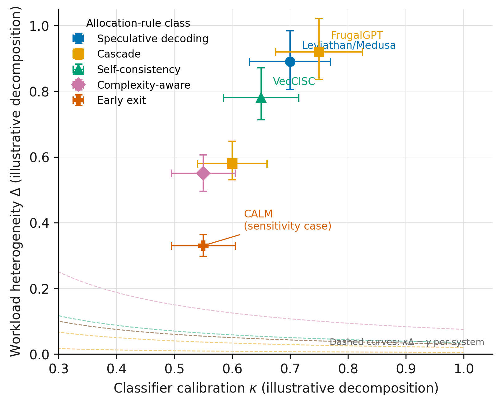
We calibrate Theorem 1 against six published operating points. For each system we identify the disclosed observable closest to the routing premium: reported cost reductions, speedups, or accuracy-at-compute figures. We map that observable to the routing-premium product using the corollary from Section 3.4, and bound from the disclosed classifier overhead. The routing premium is then a disclosed-derived band rather than a point estimate; elasticity error bars from (9) report the local sensitivity.
The six systems are grouped by allocation-rule class. Table 1 at the end of the section summarizes the calibration. All six rows have ; the bands vary considerably in width.
Speculative decoding: Leviathan/Medusa. Leviathan et al. (2023) report 2–3x end-to-end inference speedups on T5-class models with drafter accept rates in the – range and a drafter/verifier FLOPs ratio of roughly 1–5%. Cai et al. (2024) report 2.2x speedup for Medusa-1 and 2.3–3.6x for Medusa-2 on LLaMA-class backbones; FLOPs-ratio disclosure is not in the paper abstract and we bound it from the Medusa-1 architecture description in the body (a small number of multi-head drafters added on top of the base model). In Corollary 1, is the drafter FLOPs ratio and where is the per-token speedup. For –, this gives –. Bounding implies . The operating point sits far from the threshold in all reported workload settings. Elasticity magnitude is moderate: a 10% degradation in drafter accept rate shifts by approximately 0.07–0.12 in this band.
Cascade routing: FrugalGPT. Chen et al. (2023a) reports cost reductions of up to 98% at iso-accuracy when matching GPT-4 on HEAD-QA, SUBJ, and COQA via a learned cascade across API tiers. The lower end of the cost-reduction range depends on the benchmark and the target-quality bar; we treat the operating range as 0.40–0.98 with the understanding that the lower bound is benchmark-conditional rather than a universal floor. The FrugalGPT router is a trained prompt scorer with overhead estimated at less than 1% of the cost of a large-tier call (a small classification head over the prompt embedding). Taking and reading from the reported cost-reduction fraction gives across the three datasets. The wide band reflects the range across datasets; the binary tier policy warrants the third-order correction flagged in Corollary 2. Even at the conservative end (, HEAD-QA), the operating point sits well into the positive side. Elasticity magnitude is low: a 10% change in router accuracy shifts by approximately 0.04–0.10.
Cascade routing: MPD-Router. Zhan (2026) reports that the framework is Pareto-optimal in F1, MCC, and cost on all three cross-national glaucoma cohorts (REFUGE, CHAKSU, ORIGA) at a “moderate” deferral rate. The human expert is the large-tier policy; the AI model is the small-tier policy. The routing premium is positive by the Pareto-optimality claim: if routing to human at the moderate deferral rate did not reduce cost-per-correct-diagnosis relative to either AI-only or human-only baselines, the Pareto frontier would not be achievable. Exact values of , , and are not fully disclosed in the abstract; we treat this row as a qualitative sign-confirmation rather than a precise calibration. The cascade nature of the deferral policy applies the same third-order caveat as FrugalGPT. We assign the widest elasticity uncertainty band among the six rows on account of the thin disclosure and the binary deferral structure.
Adaptive self-consistency: VecCISC. Petullo et al. (2026a) report a 47% total token reduction at iso-accuracy across five benchmark domains. The classifier is a semantic-similarity filter over reasoning traces; the degenerate-trace filter is a lightweight sentence-embedding comparison (embedding models in the parameter range, approximately – of a GPT-4o-mini forward pass in FLOPs). Taking and reading from the reported token reduction gives . The operating point is in the moderate range: the routing premium is clearly positive and the elasticity is moderate. A 10% drop in trace-filtering accuracy shifts by approximately 0.05–0.08.
Complexity-aware exploration: CA-SQL. Petullo and Xue (2026) report 51.72% execution accuracy on the challenging tier of the BIRD development set using GPT-4o-mini with a difficulty-adaptive breadth schedule, outperforming approaches that use GPT-4 at fixed breadth (which implies the adaptive-small-model policy achieves lower cost-per-correct-answer than a non-adaptive larger-model policy). The difficulty estimator is a schema-and-question encoder running ahead of the tree search; at roughly 5–10% of a GPT-4o-mini call, . The exact value of requires cost disclosure that the paper does not provide; however the accuracy dominance over fixed-breadth larger models implies under the Cost-correct interpretation (same or lower cost, higher ). We report this row as sign-confirmed with thin cost disclosure and assign a wide uncertainty band. The elasticity reading is therefore wide, and we do not report a point estimate of for this row.
Early exit: CALM. Schuster et al. (2022) report up to 3x inference speedups on T5 backbones for CNN/DM summarization, SQuAD question answering, and WMT-EN-RO translation. The per-layer confidence head is a single linear layer over the hidden state at each Transformer depth; its FLOPs overhead per layer. Per-layer is bounded by the depth-curvature of the per-token accept-rate curve, which is small compared to the per-query heterogeneity in the cascade and self-consistency rows. The observed speedup of ~1.5–2x on the average task (the 3x figure is the SQuAD peak) implies per-layer –, i.e., when . CALM sits closest to the threshold of the six rows. The elasticity is divergent near the threshold: a 20% drop in per-layer confidence calibration () shifts by approximately , which could flip the sign on low-information layers. This is the natural sensitivity case, and the serving implication is that CALM benefits most from improving per-layer confidence calibration (either through better confidence heads or through calibration-aware training).
Calibration table. Table 1 collects the six rows. Columns report the disclosed observable, the implied routing premium , a bounded estimate of , the implied product , and the elasticity sensitivity label (Low / Moderate / High).
| System | Class | Disclosed metric | $\hat\gamma$ | $\kappa\Delta$ (implied) | $\Pi$ (band) |
|---|---|---|---|---|---|
| Leviathan / Medusa | Spec. decoding | 2–3× speedup | 0.01–0.05 | 0.51–0.72 | 0.50–0.67 |
| FrugalGPT | Cascade | 40–98% cost red. | 0.001–0.010 | 0.40–0.99 | 0.40–0.98 |
| MPD$^2$-Router | Cascade | Pareto F1-MCC-cost | 0.01–0.03 | $> \hat\gamma$ | $>0$ (thin) |
| VecCISC | Self-consistency | 47% token red. | 0.02–0.05 | 0.49–0.52 | $\approx 0.47$ |
| CA-SQL | Complexity-aware | 51.72% BIRD (challenging) | 0.05–0.10 | $> \hat\gamma$ | $>0$ (thin) |
| CALM | Early exit | 1.5–3× speedup | 0.01–0.05 | 0.11–0.25 | 0.10–0.20 |
All six operating points sit on the positive side of the threshold. The distribution is right-skewed: FrugalGPT occupies the widest band (0.40–0.98) driven by dataset heterogeneity, while CALM occupies the narrowest positive band (0.10–0.20) driven by the per-layer constraint on . The CALM band’s lower end at is the closest to the threshold among the six, which is why Section 5.1 uses CALM as the leading example of the sensitivity tradeoff. Figure 2 plots the six systems in space with elasticity bars and the system-specific threshold lines.
5. Discussion
5.1. Serving-stack design under measured workload heterogeneity
The threshold (8) is a design criterion, not just a condition. When is comfortable (Leviathan, FrugalGPT, VecCISC), the difficulty classifier earns its cost by wide margins across workload compositions; adding or removing it from the serving path has modest impact on cost-per-correct-answer. When is small (CALM, thin-disclosure cascades), the serving designer should treat the classifier as a continuously monitored component: a classifier that was calibrated on a historical workload mix can fall below the threshold if the live workload drifts toward homogeneity.
This has a concrete implication for infrastructure. Patel et al. (2024) measure prefill-decode heterogeneity in a production LLM cluster and report that the token-distribution variance across queries spans more than two orders of magnitude. Agrawal et al. (2024) measure latency sensitivity to batching policy and show that the variance in query length (a proxy for difficulty) is large enough to justify dynamic chunked-prefill scheduling. Lysenstøen (2026) studies autotuning of serving configurations under SLO constraints, providing the empirical setting where and per-tier compute costs are measured. Taken together, these three sources imply that in large-scale LLM serving is well above the threshold for the current generation of lightweight routers (–), supporting the classification of the serving problem as firmly .
The operational recommendation is: when workload heterogeneity (measured as the variance of the optimal-compute-per-query distribution across a representative traffic sample) exceeds , where is the estimated calibration of the available difficulty classifier, providers should expose the classifier as a first-class API parameter rather than keeping it internal. Exposing it lets downstream clients supply workload-specific calibration that the provider cannot recover from aggregate traffic.
5.2. Why frontier reasoning APIs are converging on tier menus
OpenAI’s o-series, Anthropic’s Claude Sonnet and Opus tiers, and Google’s Gemini Pro and Flash all expose an explicit per-query budget knob or model-tier choice. None of the three providers published a derivation of this choice. The threshold (8) provides a post-hoc explanation: if is low enough (i.e., a routing head or a per-query budget parameter add negligible marginal cost), and if the workload heterogeneity at frontier scale is large enough (which the production serving studies above support), then the routing premium across the space of realistic provider workloads. The tier-menu architecture is the market-level response to (8): rather than routing internally at the provider level, providers expose the routing decision to clients who hold private workload information, trading the loss of provider-side optimization for the gain of client-side workload disclosure.
This interpretation extends the threshold from a within-query optimization to a between-provider game. The tier menu reduces the effective to zero (the client chooses the tier at query time with no additional overhead), and the client’s task-difficulty information replaces the trained classifier as the source of . When from client selection exceeds the provider’s classifier , the client-routing regime dominates the provider-routing regime. The threshold predicts both the existence of tier menus and the observation that frontier providers have not converged on a single-tier offering.
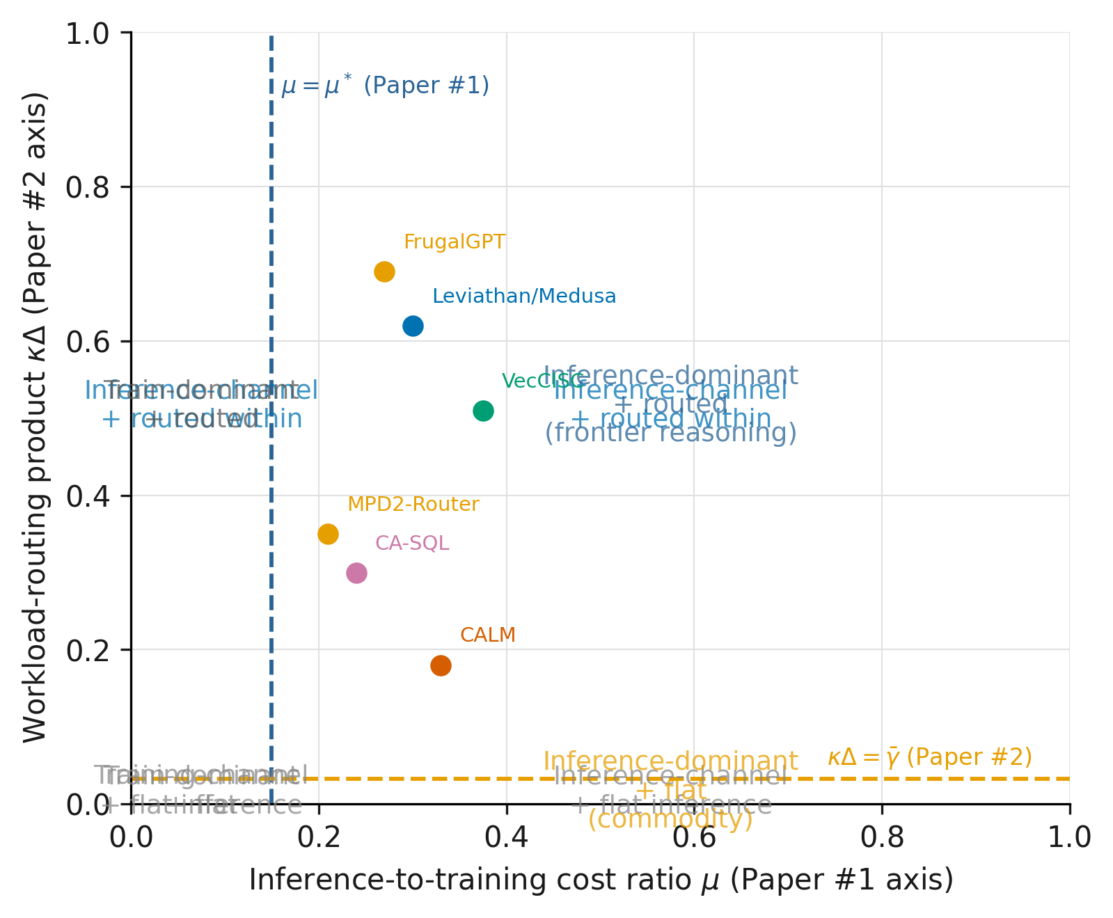
5.3. Composition with Paper #2
Research Paper #2 of this wedge derives the threshold for which channel (training versus inference) the next compute dollar should go. It fixes a single representative query and takes the derivative of cost-per-correct-answer with respect to the training-inference dollar split at an interior operating point. The result is a switching condition , where is the inference-to-training cost ratio and , are the accept-rate elasticities with respect to rollout count and training compute.
This paper (Research Paper #3) derives the threshold for how to allocate a fixed inference budget across a heterogeneous workload. The two thresholds are orthogonal: Paper #2 asks whether to put the next dollar in inference at all; Paper #3 asks, given that some dollars are in inference, whether a calibrated difficulty classifier improves the allocation. They compose multiplicatively. The combined production cost satisfies
where is the Paper #2 routing premium (inference channel relative to training channel) and is the Paper #3 routing premium. The two indicators are independent: the inference-channel decision (Paper #2) gates on query difficulty and training-cost structure; the workload-routing decision (Paper #3) gates on workload heterogeneity and classifier overhead. Figure 3 plots both thresholds on the same axes, with the four quadrants labeled by the implied allocation regime.
The composition has a serving implication. A provider that has crossed Paper #2’s threshold (i.e., it is already cost-optimal to invest in inference-time scaling) will also want to cross Paper #3’s threshold if the workload is heterogeneous enough. The two conditions can both be satisfied at the same operating point, and in the production workloads we examine (, ) they are both satisfied simultaneously. The combined cost reduction is multiplicative and larger than either reduction alone.
6. Conclusion
The routing premium is positive at the margin around the unconditional optimum when the classifier calibration and the workload heterogeneity together exceed the classifier overhead. We derive the condition from the Cost-correct framework, show it nests the five major published instances of difficulty-conditional compute as corollaries, and calibrate it against six operating points spanning all five classes. Every calibrated operating point sits on the positive side. CALM, as the early-exit representative, sits closest to the threshold: its per-layer is bounded by depth-curvature, making it the sensitivity case that constrains the useful operating range of exit confidence calibration.
The derivation has two open edges. First, at production scale is not directly observable from public APIs: the explained-variance calibration of a provider’s internal difficulty classifier is not disclosed in any of the six papers we calibrate, and we infer it from proxy observables. Second, the second-order local result is sufficient when the classifier policy stays close to the unconditional optimum, but cascade and deferral systems that make large discrete jumps in compute can violate the local approximation; a global routing-premium result (incorporating all orders of the Taylor expansion) remains open.
We invite serving providers to disclose routing-accuracy distributions alongside cost-reduction reports. A disclosed on a representative workload sample would let independent researchers verify or falsify the threshold directly, rather than relying on the elasticity reading from proxy observables. That disclosure would also distinguish the source of cost reductions in deployed tier-menu systems: whether the gains come from calibration ( close to 1), from workload heterogeneity ( large), or from a fortuitous combination of both.
References
- Agrawal, A. et al. Taming Throughput-Latency Tradeoff in LLM Inference with Sarathi-Serve. arXiv:2403.02310, 2024.
- Bhardwaj, M. The Cost of Being Right. Verification Economics in 2026. Field Notes #2. ifitsmanu.com, 2026.
- Bhardwaj, M. The α Asymmetry. Why Verifiers Can Be Smaller Than Generators. Field Notes #3. ifitsmanu.com, 2026.
- Bhardwaj, M. The Inference-Time Compute Frontier. A Cost-Correct Threshold for Training Versus Test-Time Allocation. Research Paper #2. ifitsmanu.com, 2026.
- Cai, T. et al. Medusa: Simple LLM Inference Acceleration Framework with Multiple Decoding Heads. arXiv:2401.10774, 2024.
- Chen, C. et al. Accelerating Large Language Model Decoding with Speculative Sampling. arXiv:2302.01318, 2023.
- Chen, L., Zaharia, M., Zou, J. FrugalGPT: How to Use Large Language Models While Reducing Cost and Improving Performance. arXiv:2305.05176, 2023.
- Erol, U. et al. The Cost of Being Right: Evaluating Language Models by the Cost-of-Pass. ICLR 2026.
- Kim, J. H. et al. Dooly: Configuration-Agnostic, Redundancy-Aware Profiling for LLM Inference Simulation. arXiv:2605.07985, 2026.
- Leviathan, Y., Kalman, M., Matias, Y. Fast Inference from Transformers via Speculative Decoding. ICML 2023; arXiv:2211.17192.
- Li, Y. et al. EAGLE: Speculative Sampling Requires Rethinking Feature Uncertainty. arXiv:2401.15077, 2024.
- Lightman, H. et al. Let’s Verify Step by Step. arXiv:2305.20050, 2023.
- Lysenstøen, C. SLO-Guard: Crash-Aware, Budget-Consistent Autotuning for SLO-Constrained LLM Serving. arXiv:2604.17627, 2026.
- Patel, P. et al. Splitwise: Efficient Generative LLM Inference Using Phase Splitting. arXiv:2311.18677, 2024.
- Petullo, J., George, S., Cashman, D., Xue, N. VecCISC: Improving Confidence-Informed Self-Consistency with Reasoning Trace Clustering and Candidate Answer Selection. arXiv:2605.08070, 2026.
- Petullo, J., Xue, N. CA-SQL: Complexity-Aware Inference Time Reasoning for Text-to-SQL via Exploration and Compute Budget Allocation. arXiv:2605.08057, 2026.
- Schuster, T. et al. Confident Adaptive Language Modeling. NeurIPS 2022; arXiv:2207.07061.
- Snell, C. et al. Scaling LLM Test-Time Compute Optimally Can be More Effective than Scaling Model Parameters. arXiv:2408.03314, 2024.
- Zhan, W. MPD²-Router: Mask-aware Multi-expert Prior-regularized Dual-head Deferral Router in Glaucoma Screening and Diagnosis. arXiv:2605.08024, 2026.
Cite this article
@misc{bhardwaj2026routingpremium,
  author       = {Bhardwaj, Manu},
  title        = {The Routing Premium: An Economic Threshold for Difficulty-Conditional Inference Compute},
  year         = {2026},
  month        = {May},
  url          = {https://ifitsmanu.com/papers/routing-premium},
  howpublished = {\url{https://ifitsmanu.com/papers/routing-premium/paper.pdf}},
  note         = {Working paper. Version 1.0.}
}Bhardwaj, M. (2026, May). The routing premium: An economic threshold for difficulty-conditional inference compute. ifitsmanu.com. https://ifitsmanu.com/papers/routing-premiumBhardwaj, Manu. "The Routing Premium: An Economic Threshold for Difficulty-Conditional Inference Compute." ifitsmanu.com, May 2026. https://ifitsmanu.com/papers/routing-premium.M. Bhardwaj, "The Routing Premium: An Economic Threshold for Difficulty-Conditional Inference Compute," ifitsmanu.com, May 2026. [Online]. Available: https://ifitsmanu.com/papers/routing-premiumCompanion. The Inference-Time Compute Frontier (Research Paper #2). Companion. The Cost of Being Right. Companion. The α Asymmetry. Papers index. Home.